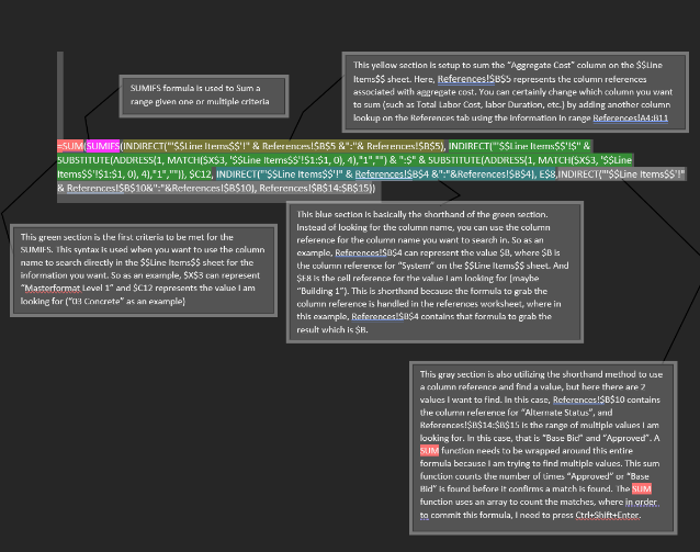
=SUM(SUMIFS(INDIRECT("'$$Line Items$$'!" & References!$B$5 &":"& References!$B$5), INDIRECT("'$$Line Items$$'!$" & SUBSTITUTE(ADDRESS(1, MATCH($X$3, '$$Line Items$$'!$1:$1, 0), 4),"1","") & ":$" & SUBSTITUTE(ADDRESS(1, MATCH($X$3, '$$Line Items$$'!$1:$1, 0), 4),"1","")), $C12, INDIRECT("'$$Line Items$$'!" & References!$B$4 &":"&References!$B$4), E$8,INDIRECT("'$$Line Items$$'!" & References!$B$10&":"&References!$B$10), References!$B$14:$B$15))
SUMIFS - SUMIFS formula is used to Sum a range given one or multiple criteria
(INDIRECT("'$$Line Items$$'!" & References!$B$5 &":"& References!$B$5), - This yellow section is set up to sum the “Aggregate Cost” column on the $$Line Items$$ sheet. Here, References!$B$5 represents the column references associated with aggregate cost. You can certainly change which column you want to sum (such as Total Labor Cost, labor Duration, etc.) by adding another column lookup on the References tab using the information in range References!A4:B11
INDIRECT("'$$Line Items$$'!$" & SUBSTITUTE(ADDRESS(1, MATCH($X$3, '$$Line Items$$'!$1:$1, 0), 4),"1","") & ":$" & SUBSTITUTE(ADDRESS(1, MATCH($X$3, '$$Line Items$$'!$1:$1, 0), 4),"1","")), $C12 -
This green section is the first criteria to be met for the SUMIFS. This syntax is used when you want to use the column name to search directly in the $$Line Items$$ sheet for the information you want. So as an example, $X$3 can represent “Masterformat Level 1” and $C12 represents the value I am looking for (“03 Concrete” as an example)
INDIRECT("'$$Line Items$$'!" & References!$B$4 &":"&References!$B$4), E$8 -
This purple section is basically the shorthand of the green section. Instead of looking for the column name, you can use the column reference for the column name you want to search in. So as an example, References!$B$4 can represent the value $B, where $B is the column reference for “System” on the $$Line Items$$ sheet. And $E8 is the cell reference for the value I am looking for (maybe “Building 1”). This is shorthand because the formula to grab the column reference is handled in the references worksheet, where in this example, References!$B$4 contains that formula to grab the result which is $B.
INDIRECT("'$$Line Items$$'!" & References!$B$10&":"&References!$B$10), References!$B$14:$B$15) -
This blue section is also utilizing the shorthand method to use a column reference and find a value, but here there are 2 values I want to find. In this case, References!$B$10 contains the column reference for “Alternate Status”, and References!$B$14:$B$15 is the range of multiple values I am looking for. In this case, that is “Base Bid” and “Approved”. A SUM function needs to be wrapped around this entire formula because I am trying to find multiple values. This sum function counts the number of times “Approved” or “Base Bid” is found before it confirms a match is found. The SUM function uses an array to count the matches, where in order to commit this formula, I need to press Ctrl+Shift+Enter