**Note that all Dashboard editing is most efficiently handled working directly in Excel. Hit Save As… inside of Estimator’s Dashboard view to create that Excel file.
**Note that this article builds on the concepts shown in Advanced Dashboard Logic – How to use a SUMIFS statement article
Tying a formula directly to a specific cell or column in Excel is acceptable when working in a static data environment. However, Estimator’s Dashboard creates $$____$$ sheets that are dynamic and constantly updating. For example, if a new WBS is added to the estimate, the $$Line Items$$ sheet reorders the WBS columns in ABC order. If you wrote a formula based on a specific column, you could end up with #REF errors or invalid data results when you introduce a new WBS.
To protect against this scenario, a full-fledged Dashboard can utilize a References sheet. This allows us to use additional excel logic to dynamically seek out specific WBS and update their column location in the associated formulas.
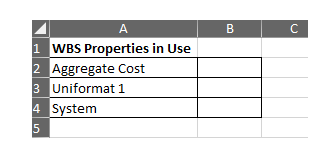
Create a new tab in your Excel workbook and name it References.
On that page, create a small list like the one shown below for your desired WBS properties.
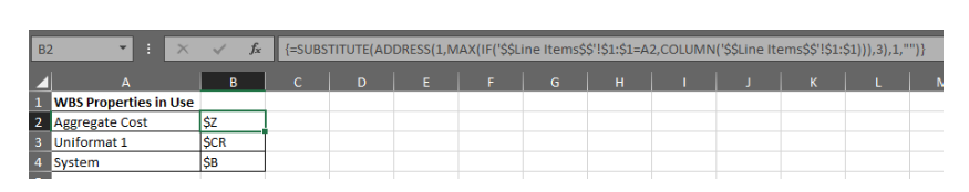
You can either manually update these cells as data changes, OR use a fancy formula to do it for you automatically. If you choose option 2, you can use the formula below and paste it into cell B2. Because it is an array formula, you’ll need to click into the cell and hit CTRL+SHIFT+ENTER to activate the “magic”. It will add { } brackets for you automatically.
=SUBSTITUTE(ADDRESS(1,MAX(IF('$$Line Items$$'!$1:$1=A2,COLUMN('$$Line Items$$'!$1:$1))),3),1,"")
Whichever route you choose, you should see something like the results below.
The end goal here is that instead of saying our aggregate total range is …
'$$Line Items$$'! $Z:$Z
we will instead introduce a dynamic environment...
INDIRECT('$$Line Items$$'! (References Tab, Cell B3) : (References Tab, Cell B3))
The INDIRECT function returns the value of a cell that contains the text called out in the equation. We will basically be using it as an advanced CONCATENATE function. As such, the string sections will be brackets by "____" and joined by the & symbol.
INDIRECT( " ' Page Name ' ! " + "References Cell" + ":" + References Cell)
Line Item Aggregate Total
INDIRECT("'$$Line Items$$'!" & References!$B$2 & ":" & References!$B$2)
=
'$$Line Items$$'!$Z:$Z
Uniformat Level 1
INDIRECT("'$$Line Items$$'!" & References!$B$3 & ":" & References!$B$3)
=
'$$Line Items$$'!$BP:$BP
System
INDIRECT("'$$Line Items$$'!" & References!$B$4 & ":" & References!$B$4)
=
'$$Line Items$$'!$B:$B
Note: The $ on the column names locks that reference location, no matter where the formula is pasted. Formulas in excel are by default relative, so we are overriding that.
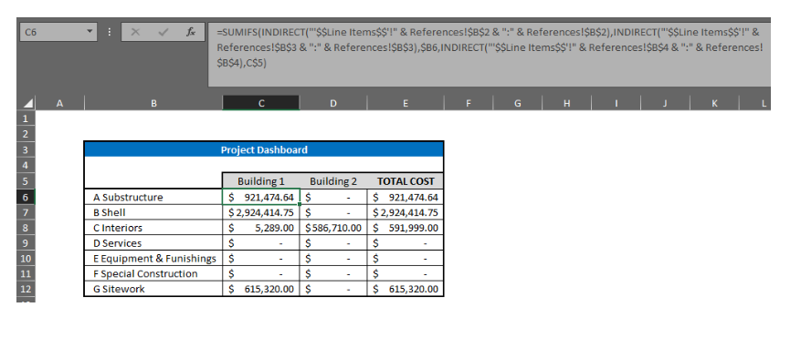
The end result is the new SUMIFS formula for that cell. Replacing the hard-coded ranges with dynamic ones, and keeping the same criteria for each criteria range.
=SUMIFS(INDIRECT("'$$Line Items$$'!" & References!$B$2 & ":" & References!$B$2),INDIRECT("'$$Line Items$$'!" & References!$B$3 & ":" & References!$B$3),$B6,INDIRECT("'$$Line Items$$'!" & References!$B$4 & ":" & References!$B$4),C$5)