Advanced Dashboard Logic - How to use a SUMIFS Statement
**Note that all Dashboard editing is most efficiently handled by working directly in Excel. Hit Save As… inside of Estimator’s Dashboard view to create that Excel file.
GOAL: Sum up the aggregate cost of line items that meet specific criteria in a single cell.
The SUMIFS function will sum up the selected cells if all criteria in the equation, whether ONE or MULTIPLE, are met.
=SUMIFS(Sum Range, Criteria Range 1, Criteria 1, Criteria Range 2, Criteria 2, …)
Or in plain English…
=SUMIFS(Sum THIS Column, if this criteria is met, and that criteria is met, etc)
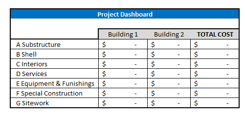
This dashboard displays the total cost per Uniformat 1 division, broken out by “System” name.

On the $$Line Items tab, our data source for this dashboard, I looked for these columns:
System = B
Uniformat 1 = CR
Aggregate Cost = Z
Time to write the formula for Cell C6:
In English: Sum the Aggregate Cost for all Building 1 Items in “A Substructure”.
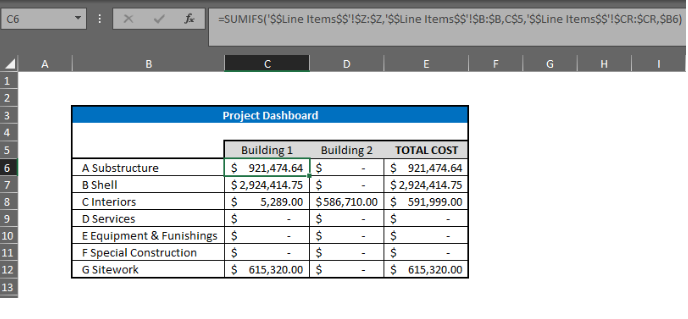
In Excel: SUMIFS('$$Line Items$$'!$Z:$Z, '$$Line Items$$'!$B:$B, C$5, '$$Line Items$$'!$CR:$CR, $B6)
You can then drag that formula down for the rest of the rows in Column C, and also drag it to cover Column B.
Note: The $ symbol in the C$5 and $B6 “criteria” cells are important. That creates an absolute reference, locking the row number and column respectively, which allows us to write a single formula and then drag it down/over to fill the rest of the dashboard.
Here is the dashboard with the logic copied to all cells:
